Time Series Analysis

The Time Series Analysis widget enables users to independently investigate time series data with flexibility, within the framework of the Workshop application.

Available plots

Add time series data from the Ontology with the + Add Data search bar, then derive new plots by selecting New Plot. Plots can be organized across multiple canvases within the same analysis.

Time series plots

• Bollinger bands: Plot upper and lower bands at a configurable number of standard deviations around a moving average.
• Combine time series: Merge multiple time series into a single plot, specifying how to handle overlapping time points (for example, mean, min, or max).
• Cumulative aggregate: Display the cumulative value of a series over the entire length of the series or over a specific period of time.
• Derivative: Display the rate of change at each point in the selected input series.
• DSP filter: Apply a digital signal processing filter (Butterworth, Chebyshev, or inverse Chebyshev) to reduce noise in a time series.
• Event statistics: Aggregate a time series over intervals where an event occurs, returning one point per event.
• Filter time series: Keep or remove points in a time series based on a time range or mathematical condition.
• Formula time series: Create a new plot by applying a mathematical formula across one or more time series using Quiver's formula language.
• Integral: Calculate the area under the curve of a time series, the inverse of a derivative.
• Linear aggregation: Compute a linear aggregation across multiple time series over time.
• Periodic aggregate: Downsample a time series by aggregating data over fixed time periods, producing one point per period.
• Rolling aggregate: Calculate a new point for each data point based on a rolling window function and aggregate method, typically used to smooth a series.
• Sample: Resample a time series at a constant frequency to fill gaps or change the data rate.
• Shift time series: Shift the time of a series forwards or backwards by a specified duration.

Event sets

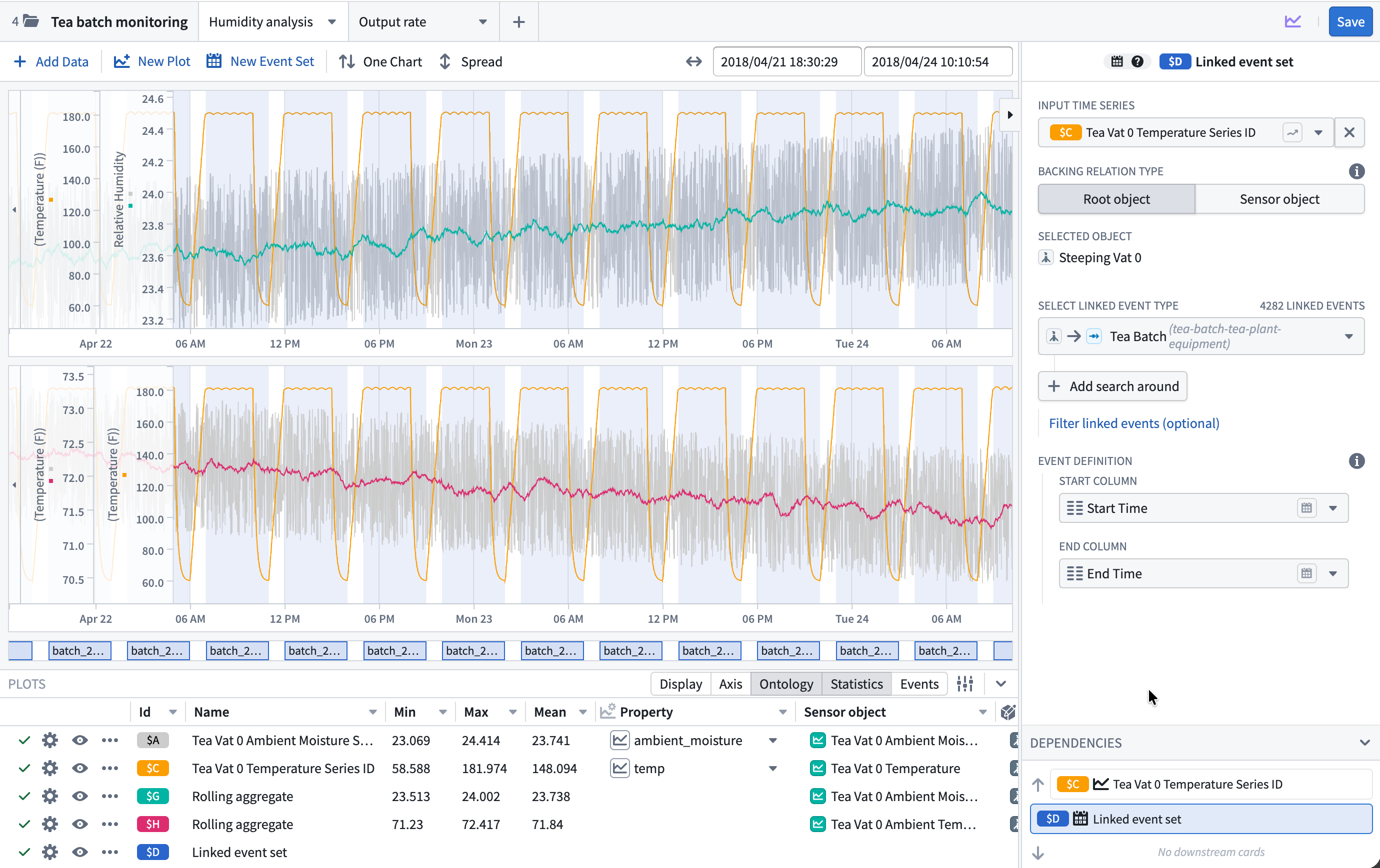
• Linked event set: Create an event set from linked objects in the Ontology by traversing object relationships and specifying which properties hold the start and end timestamps.
• Time series search: Create an event set from conditions on time series data, identifying time ranges that match a specified pattern or threshold.

Visualization options

The Plots panel at the bottom of the widget contains settings and information that are common to all plot types. Data configurations specific to the plot type are controlled in the editor panel on the right side of the widget. Column visibility, ordering, sorting, and widths are all customizable. Use the Configure columns menu for fine-grained control of the column ordering and to add non-default columns.

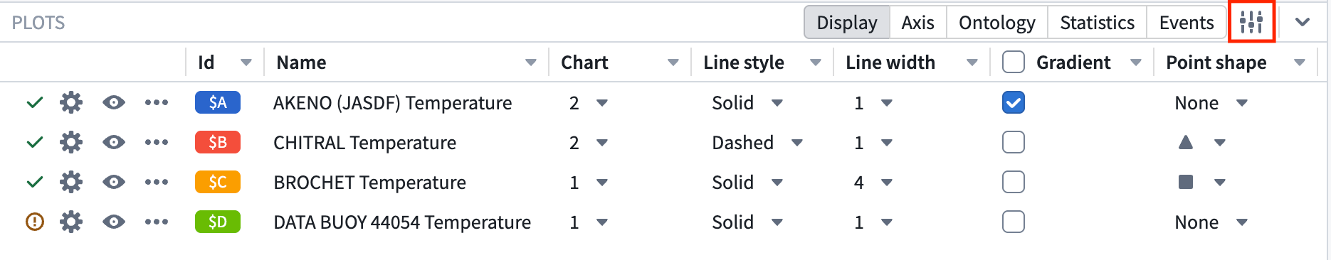
The following visualization options can be quickly toggled from the panel header:

Display

• Chart: The canvas chart that the plot is rendered on.
• Line style: Render the plot line as solid or dashed.
• Line width: The thickness of the plot line.
• Gradient: Toggle gradient shading under the plot line.
• Point shape: The shape of data points (circle, triangle, square, diamond, or none).
• Point size: The size of data points. Disabled when point shape is set to none.

Axis

• Axis: The Y-axis assignment for the plot. Select from existing axes with a compatible unit, or create a new axis.
• Unit: The unit of the Y-axis. Allows unit conversion (for example, meters to kilometers) or custom label overrides.
• Auto scale: Toggle automatic axis scaling to fit the data extent.
• Axis min: The minimum value of the Y-axis range. Disabled when auto scale is active.
• Axis max: The maximum value of the Y-axis range. Disabled when auto scale is active.

Ontology

• Root object: The Ontology object that the time series property is located on, or the root object if the time series is a sensor. Selecting a different object updates the plot and any dependent derived plots. When all plots have the same root object, this column can be bulk updated using the button in the column header.
• Sensor object: The sensor object associated with the time series (if applicable).
• Property: The time series property or sensor name. Selecting a different property updates the plot and any dependent derived plots. When all plots are using the same property, this column can be bulk updated using the button in the column header.

Statistics

• Min: The minimum value of the plot within the current view range.
• Max: The maximum value of the plot within the current view range.
• Mean: The mean value of the plot within the current view range.

Events

• Event count: The number of events within the current view range for event set plots.
• Event highlight: Toggle chart highlighting for time ranges where events occur.

Additional configurations can be added from the Column configuration menu:

Axis display options

• Align axis: Align the axis to the left or right side of the chart.
• Log scale: Display the axis using a logarithmic scale.
• Invert axis: Invert the direction of the axis.

Point display options

• Point fill: The fill color of data points. Disabled when point shape is set to none.
• Point outline width: The outline width of data points. Disabled when point fill is set to none or is the same as the plot color.

Interpolation

• Internal interpolation: The interpolation method used to connect data points within the time series.
• External interpolation: The interpolation method used before the first data point and after the last data point.

Learn more about available interpolation options.

Configuration options

Add data options

• Enable users to select time series data from the Ontology, optionally restricting which object types are available. To further narrow the available series, apply object set filters for each object type.
• Control series with object sets: Initialize the analysis with a controlled set of time series by specifying object sets and time series properties. Users cannot delete or edit the data configuration for these series but can customize the display from the Plot Details panel.
• Add initial event sets: Initialize the analysis with event sets backed by object sets, specifying the properties to use for event start and end times. Users cannot delete or edit the data configuration for these series but can customize the display from the Plot Details panel.

Plot options

• New plot placement: Choose which canvas new plots are added to by default.
• Customize available plot types: Control which derived plot types are available from the New plot menu and the order in which they appear.
• Customize available event set types: Control which types of event sets can be added by the user.

Chart options

• Overlay Y-axes: When enabled, Y-axes are rendered as transparent overlays. Otherwise, the Y-axes will shift the chart data to the side.
• Collapse Y-axes by default: Start with Y-axes collapsed to save chart space.
• Display Y-axes boundaries when collapsed: Display axis boundaries when axes are collapsed.
• Tooltip options: Configure tooltip visibility, displayed values, time and label formatting, text wrapping, and the number of significant digits.
• Enable UTC time format: Display chart time values in UTC format.
• Sync X-axes across canvases: Keep the X-axis view range synchronized when zooming or panning across multiple canvases.
• Default view range: The initial view range for time series charts in the analysis. The available options include:
  • Full data range: Use the start and end dates of the included time series. Note that this may negatively impact performance for large time series.
  • Fixed date range: Use workshop variables to define absolute start and end dates.
  • Relative date range: Use workshop variables to define a range relative to the time when the page was loaded (for example, "2 weeks ago to now").

Resource options

• Enable analysis saving: Save and share analyses for future reference. Analyses can be saved as either Private or Public.
  • Configure default save location: Select a folder or use a string variable to provide the default save location.
  • Don't allow users to choose save location: Always use the default save location and hide the save location select in the UI.
• Output analysis RID: Store the resource identifier of the active analysis in a string variable for use elsewhere in the Workshop application.
• Autoload analyses: Specify analyses to load automatically when the widget initializes. Display options from the widget configuration (for example, tooltip options) will override those saved on the analysis, but the analysis will retain its original settings when saved from the widget.
  • Don't clear on load: When disabled, updating the autoloaded analysis RIDs will reset the widget view state. If enabled, updating the analysis RIDs will add new analyses to the view state, but will not clear analyses currently being viewed.

Save an analysis for later use

• Save as a time series analysis resource: Toggle on the Enable analysis saving configuration to allow users to preserve and easily share their analyses. Saved analyses can be opened in a standalone resource view or loaded into the Workshop widget using its RID.
• Open in Quiver: Select Open in Quiver from the upper right corner of the widget header to transfer the analysis to a full Quiver analysis for more advanced time series workflows. This creates a new Quiver analysis with the same canvases and plots. Note that changes made in the Quiver analysis are not reflected back in the Workshop widget.