Reference profiles

Reference profiles define the expected behavior of a sensor during a specific process. To construct a reference profile, a set of process runs or events, known as a golden batch, is selected, where the overall processes performed as expected. The corresponding sensor data from these runs can then be used to construct reference profile bounds, typically using the mean plus or minus n standard deviations at each time point. This range represents the expected operating window for the sensor during that process.

For example, consider the water temperature sensor during a tea steeping process that is carried out regularly under controlled conditions. By selecting batches where the steeping process completed normally, we can use the temperature data from these runs to establish upper and lower bounds for the sensor. This allows us to compare future tea steeping cycles against the reference profile to detect deviations from normal operation.

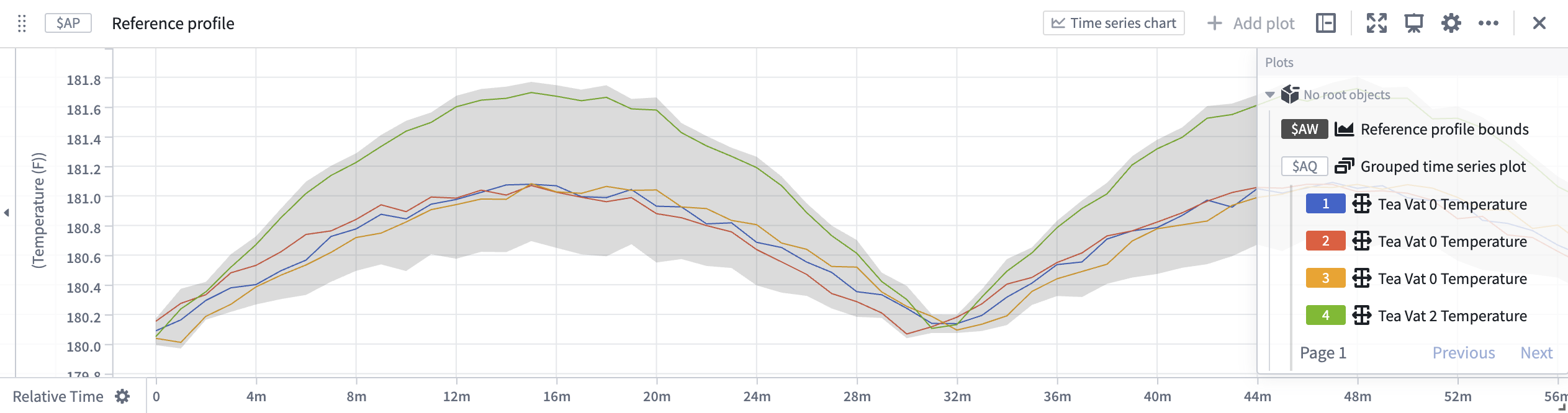
In the screenshot, the shaded area shows the expected operating range for the water temperature sensor, calculated as the average value plus or minus two times the standard deviation across the selected golden batch curves.

Reference profiles in Quiver

The reference profile bounds card enables quick construction of reference curves defined by the average plus or minus n standard deviations provided a set of curves in relative time.

The process of constructing the input series for the reference profile bounds includes:

1. Taking a sensor
2. Filtering the sensor to the time where a process (event) occurred
3. Aligning the series relative to their process start time

Event comparison card

The event comparison card enables taking a single time series and an event set, and comparing the behavior of the series during the provided events. The output of an event comparison is a grouped time series which can be used as an input to the reference profile bounds card.

See Analyze events data for other ways to construct an event set.

Transform table

To use more than one time series in reference profile construction, a transform table is required. To do this:

1. Join time series and event data in a transform table and use the filter time series transform to filter each series to the event start and end times.
2. Use the relative time series transform to align each series to the associated event start time.
3. Add a grouped time series plot card from the transform table selecting the filtered and relative aligned time series.
4. Use the reference profile bounds card with the grouped time series plot as the input.

Alternatively, you can skip the grouped time series plot if you do not need to visualize the individual filtered and relative aligned curves. In this case, you can construct a reference profile bounds card directly from the transform table.

The reference profile bounds can also be constructed manually. Follow the steps above, but instead of using a reference profile bounds card, use the linear aggregation card to select and aggregate all of the filtered and aligned time series in the transform table. Repeat these steps to construct an average and a standard deviation aggregation of the curves. Finally, use a time series formula card to create an upper ($average + (2 * $standard_deviation) and lower bound ($average - (2 * $standard_deviation). This method also enables using custom logic for defining the upper and lower bounds (e.g. rolling window bounds).

Reference profiles in derived series

Reference profile curves can be constructed for derived series and referenced from time series properties enabling consumption of the reference profiles outside of Quiver.

Recommended Ontology structure

The process for selecting a golden batch is often unique to each application, we recommend a flexible Ontology structure that enables management of reference profile metadata and the ability to construct templated derived series.

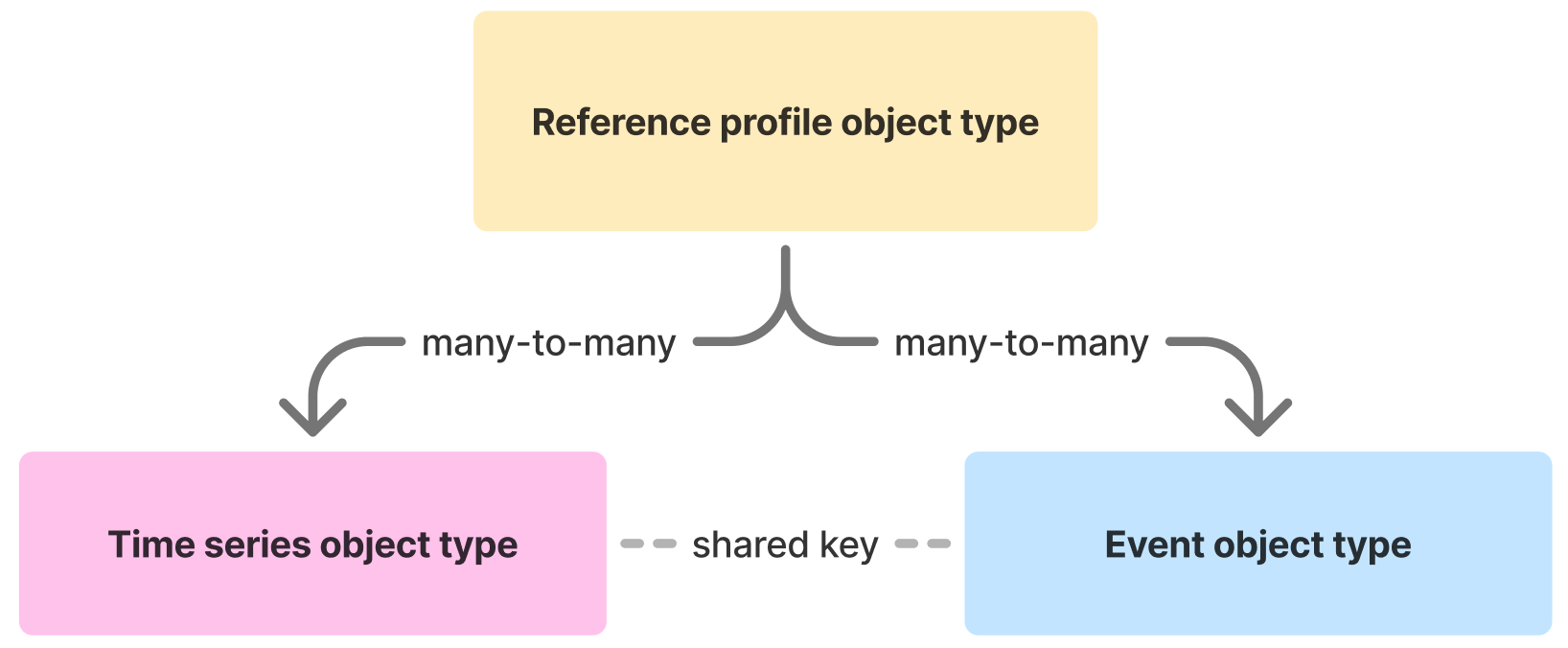
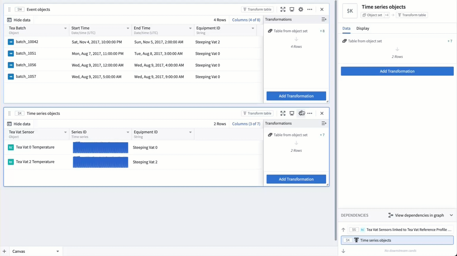
• Reference Profile Object Type: Serves as the metadata for the reference profile, linking to both the relevant time series and event objects. This will be the root object type of the derived series and will enable seamless construction of templated derived series.
• Time Series Object Type: Contains a time series property representing the sensor data to be analyzed, for example, temperature series.
• Event Object Type: Represents the process runs or batches identified as the golden batch for reference profile construction. Contains a start and end timestamp representing the time bounds of the event/process/batch.

Both the time series and event object types must share a common key (property value) to enable association. By joining these on the common key, the time series data can be assessed specifically during the associated golden batch events.

The derived series can either be referenced from time series properties on the reference profile object type or as sensor objects on a linked sensor object type.

This structure enables flexible selection and aggregation of time series data based on process events, supporting robust construction of reference profiles across a variety of applications. You can create a Workshop module to enable the management of the reference profile objects.

Derived series logic

The linked series aggregation card allows you to specify an input object and define search-around logic to gather and aggregate linked time series objects. Optionally, you can include logic to search for event objects. If event objects are provided, a common key between the time series and event objects is required. This ensures that the resulting time series are evaluated specifically during the associated events.

To construct reference profile in derived series:

1. Create two linked series aggregations aligned with events.
   • The input object should be one of the reference profile objects.
   • The first linked series will create an average aggregation and the second a standard deviation.
2. Use the time series formula card to construct an upper bound ($average + 2 * $standard_deviation) and a lower bound ($average - 2 * $standard_deviation).